In order to make full use of the Matlab interface to S-GeMS some knowledge of the use of S-GeMS is essential. The book Applied Geostatistics with SGeMS (Remy, Boucher and Wu, Cambridge University Press, 2009), written by the developers of S-GeMS is highly recommended.
The Matlab interface to S-GeMS relies on a feature of S-GeMS that allow S-GeMS to read and execute a series of Python commands from the command line, without the need to load the graphical user interface, as for example:
sgems -s sgems_python_script.py
The Matlab interface consists of methods and functions to automatically create such a Python script, execute the script using S-GeMS and load the simulated/estimated results into Matlab
One function (the section called “sgems_grid”) handles these actions allowing simulation on grids in the following manner:
Define a parameter file (the section called “sgems_get_par”, the section called “sgems_read_xml”)
Write a python script that (the section called “sgems_grid_py”)
sets up a grid or pointset where simulation or estimation is performed
performs the simulation/estimation
export the simulated/estimated data
Load the data into Matlab (the section called “sgems_write”)
For a complete list of S-GeMS related commands on mGstat see the section called “S-GeMS functions”
This section contains a rather detailed explanation of using S-GeMS to perform simulation. Much more compact example can be found in the following chapters.
Unconditional and conditional sequential simulation can be performed using the section called “sgems_grid” :
S = sgems_grid(S);
Where S is a Matlab data structure containing all the information needed to setup and run S-GeMS
A number of different simulation algorithms are available in S-GeMS The behavior of each algorithm is controlled through an XML file. Such an XML file can for example be exported from S-GeMS by choosing to save a parameter file for a specific algorithm.
Such an XML formatted parameter is needed to perform any kind of simulation. A number of 'default' parameter files available using the the section called “sgems_get_par” function. For example to obtain a default parameter file for sequential Gaussian simulation use
S = sgems_get_par('sgsim')

S =

    xml_file: 'sgsim.par'
         XML: [1x1 struct]
As can be seen the adds the name of the XML file (S.xml_file) as well as a XML data structure in the S-GeMS matlab structure S.XML.
All supported simulation/estimation types can be found calling sgems_get_par without arguments:
>> sgems_get_par
sgems_get_par : available SGeMS type dssim
sgems_get_par : available SGeMS type filtersim_cate
sgems_get_par : available SGeMS type filtersim_cont
sgems_get_par : available SGeMS type lusim
sgems_get_par : available SGeMS type sgsim
sgems_get_par : available SGeMS type snesim_std
Now all parameters for 'sgsim' simulation can be set directly from the Matlab command line. To see the number of fields in the XML file (refer to the S-GeMS book described above for the meaning of all parameters):
>> S.XML.parameters

ans =

                algorithm: [1x1 struct]
                Grid_Name: [1x1 struct]
            Property_Name: [1x1 struct]
          Nb_Realizations: [1x1 struct]
                     Seed: [1x1 struct]
             Kriging_Type: [1x1 struct]
                    Trend: [1x1 struct]
      Local_Mean_Property: [1x1 struct]
         Assign_Hard_Data: [1x1 struct]
                Hard_Data: [1x1 struct]
    Max_Conditioning_Data: [1x1 struct]
         Search_Ellipsoid: [1x1 struct]
     Use_Target_Histogram: [1x1 struct]
              nonParamCdf: [1x1 struct]
                Variogram: [1x1 struct]
To see the number of realization :
>> S.XML.parameters.Nb_Realizations

ans =

    value: 10
To set the number of realization to 20 do:
>> S.XML.parameters.Nb_Realizations.value=20;
One also need to define the grid used for simulation. This is done through the S.dim data structure:
%grid size
S.dim.nx=70;
S.dim.ny=60;
S.dim.nz=1;
% grid cell size
S.dim.dx=1;
S.dim.dy=1;
S.dim.dz=1;
% grid origin
S.dim.x0=0;
S.dim.y0=0;
S.dim.z0=0;
All the values listed above for the S.dim data structure are default, thus if they are not set, they are assumed as listed.
Unconditional simulation is now performed using:
>> S=sgems_grid(S);
sgems_grid : Trying to run SGeMS using sgsim.py, output to SGSIM.out
'import site' failed; use -v for traceback
Executing script...

working on realization 1
|#                   |    5%working on realization 2
|##                  |    10%working on realization 3
|###                 |    15%working on realization 4
|####                |    20%working on realization 5
|#####               |    25%working on realization 6
|######              |    30%working on realization 7
|#######             |    35%working on realization 8
|########            |    40%working on realization 9
|#########           |    45%working on realization 10
|##########          |    50%working on realization 11
|###########         |    55%working on realization 12
|############        |    60%working on realization 13
|#############       |    65%working on realization 14
|##############      |    70%working on realization 15
|###############     |    75%working on realization 16
|################    |    80%working on realization 17
|#################   |    85%working on realization 18
|##################  |    90%working on realization 19
|################### |    95%working on realization 20
|####################|    100%
sgems_read : Reading GRID data from SGSIM.sgems
sgems_grid : SGeMS ran successfully

S =

    xml_file: 'sgsim.par'
         XML: [1x1 struct]
         dim: [1x1 struct]
        data: [4200x20 double]
           O: [1x1 struct]
           x: [1x70 double]
           y: [1x60 double]
           z: 1
           D: [4-D double]
As seen above the following field have been added to the S-GeMS matlab structure:
S.x,
S.y,
S.z,
S.data and
S.D.
S.x,
S.y,
S.z are 3 arrays defining the grid.
S.data, is the simulated data as exported from S-GeMS. Note the each realization is returned as a list of size nx*ny*nz.
S.D, is but a rearrangement of S.data into a 4D dimensional data structure, of size (nx,ny,nz,nsim). To visualize for example the 3rd realization use for example:
imagesc(S.x,S.y,S.D(:,:,1,3));
Conditional simulation can be performed by setting the S.d_obs parameter. For example:
S.d_obs=[18 13 0 0; 5 5 0 1; 2 28 0 1];
S=sgems_grid(S);
imagesc(S.x,S.y,S.D(:,:,1,3));
Using sequential Gaussian simulation the semivariogram model is specified in
S.XML.parameters.Variogram:
>> S.XML.parameters.Variogram
ans=
      nugget: 1.0000e-003
   structures_count: 1
        structure_1: [1x1 struct
To run 10 simulations with increasing range do for example:
for i=1:1:10
  r=i*10;
  S.XML.parameters.Variogram.structure_1.ranges.max=[r];
  S.XML.parameters.Variogram.structure_1.ranges.medium=[r];
  S.XML.parameters.Variogram.structure_1.ranges.min=[r];
  S=sgems_grid(S);
  subplot(4,3,i);imagesc(S.x,S.y,S.D(:,:,1)');
end
The variogram model can also be specified using a shorter notation (same format as when using GSTAT):
S.XML.parameters.Variogram=sgems_variogram_xml('0.1 Nug(0) + 0.4 Exp(10) + 0.5 Sph(40,30,0.2)');
A simple example of unconditional sequential simulation.
S=sgems_get_par('sgsim');
S.XML.parameters.Nb_Realizations.value=12;
S=sgems_grid(S);
for i=1:S.XML.parameters.Nb_Realizations.value;
  subplot(4,3,i);
  imagesc(S.x,S.y,S.D(:,:,1,i));
end
Conditioning data can be specified either as a data variable or as an sgems-binary formatted file (see the section called “S-GeMS data format”).
A simple example of conditional sequential simulation (examples/sgems_examples/sgems_example_sgsim_conditional.m):
% sgems_sgsim_conditional :
%     Conditional SGSIM using hard data from variable

% GET Default par file
S=sgems_get_par('sgsim');

% Define observed data=
S.d_obs=[18 13 0 0; 5 5 0 1; 2 28 0 1];

S.XML.parameters.Nb_Realizations.value=10;
S=sgems_grid(S);

% PLOT DATA
cax=[-2 2];
for i=1:S.XML.parameters.Nb_Realizations.value;
  subplot(4,3,i);
  imagesc(S.x,S.y,S.D(:,:,1,i)');axis image;caxis(cax);title(sprintf('SIM#=%d',i))
end

print('-dpng','sgems_sgsim_conditional')
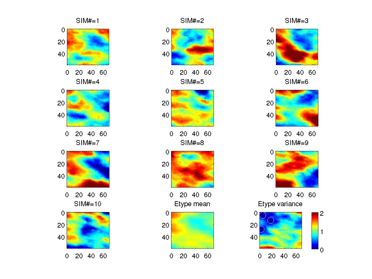
A simple example of conditional sequential simulation (examples/sgems_examples/sgems_example_sgsim_conditional_hard_data_from_file.m):
% sgems_sgsim_conditional_hard_data_from_file :
%     Conditional SGSIM using hard data from file

% GET Default par file
S=sgems_get_par('sgsim');

% Define observed data=
d_obs=[18 13 0 0; 5 5 0 1; 2 28 0 1];
sgems_write_pointset('obs.sgems',d_obs);
S.f_obs='obs.sgems';

S.XML.parameters.Nb_Realizations.value=10;
S=sgems_grid(S);


%% PLOT DATA
cax=[-2 2];
for i=1:S.XML.parameters.Nb_Realizations.value;
  subplot(4,3,i);
  imagesc(S.x,S.y,S.D(:,:,1,i)');axis image;caxis(cax);title(sprintf('SIM#=%d',i))
end
[m,v]=etype(S.D);
subplot(4,3,11);
imagesc(S.x,S.y,m');axis image;caxis(cax);title('Etype mean')
subplot(4,3,12);
imagesc(S.x,S.y,v');axis image;caxis([0 2]);title('Etype variance')
hold on
plot(d_obs(:,1),d_obs(:,2),'wo','MarkerSize',10)
hold off
colorbar

print('-dpng','sgems_sgsim_conditional_hard_data_from_file')
 |
Sequential Gaussian conditional simulation
A simple example of unconditional SNESIM AND FILTERSIM simulation.
S1=sgems_get_par('snesim_std'); %
% Note that S1.ti_file is automatically set.
% simply change this to point to another training to use.
S1.XML.parameters.Nb_Realizations.value=4;

S2=sgems_get_par('filtersim_cont');
S2.XML.parameters.Nb_Realizations.value=4;

S1=sgems_grid(S1);
S2=sgems_grid(S2);


for i=1:S1.XML.parameters.Nb_Realizations.value;
  subplot(S1.XML.parameters.Nb_Realizations.value,2,i);
  imagesc(S1.x,S1.y,S1.D(:,:,1,i));axis image;

  subplot(S1.XML.parameters.Nb_Realizations.value,2,i+S1.XML.parameters.Nb_Realizations.value);
  imagesc(S2.x,S2.y,S2.D(:,:,1,i));axis image;
end
Using a JPG file from FLICKR as training image:
% sgems_example_to_from_image : convert image and use as training image

% LOAD IMAGE AND CONVERT TO SGeMS binary TRAINING IMAGE
%file_img='1609350318_7300f07360_m_d.jpg'; % larger pattern
file_img='1609350318_7300f07360_m_d.jpg'; % smaller pattern
f_out=sgems_image2ti(file_img);
TI=sgems_read(f_out);


% SETUP FILTERSIM
S=sgems_get_par('filtersim_cont');
S.ti_file=f_out;
S.XML.parameters.PropertySelector_Training.grid=TI.grid_name;
S.XML.parameters.PropertySelector_Training.property=TI.property{1};
S.XML.parameters.Nb_Realizations.value=1;


S.dim.x=[1:1:200];
S.dim.y=[1:1:200];
S.dim.z=[0];

% RUN SIMULATION
S=sgems_grid(S);


% VISUALIZE RELIZATION
subplot(1,2,1);
imagesc(TI.x,TI.y,TI.D(:,:,:,1)');axis image;
subplot(1,2,2);
imagesc(S.x,S.y,S.D(:,:,:,1)');axis image;

print('-dpng','sgems_example_ti_from_image');
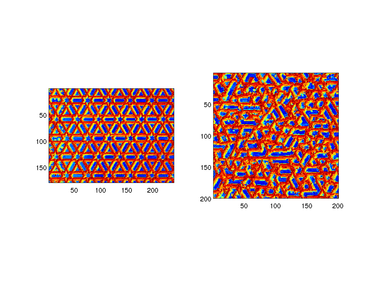 |
Example of converting an image and using it for continuous filtersim simulation
Demonstration simulation of mGstat supported simulation algorithms can be performed using the section called “sgems_demo”. To see a list of supported simulation algorithms use:
>> sgems_get_par
sgems_get_par : available SGeMS type dssim
sgems_get_par : available SGeMS type filtersim_cate
sgems_get_par : available SGeMS type filtersim_cont
sgems_get_par : available SGeMS type lusim
sgems_get_par : available SGeMS type sgsim
sgems_get_par : available SGeMS type snesim_std
To run a demonstration of continuous filtersim simulation using the 'filtersim_cont' algorithm do
>> sgems_demo('filtersim_cont');
This will perform both unconditional and conditional simulation, and visualize the results as for example here below.
 |
Unconditional simulation
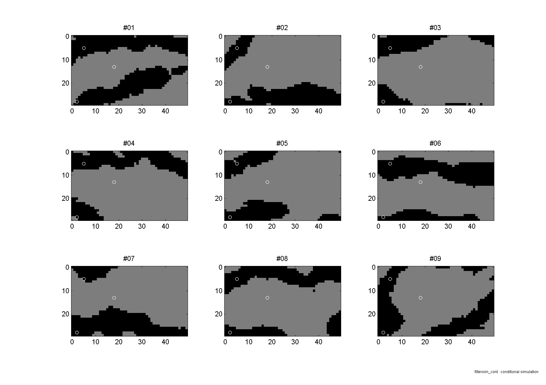 |
Conditional simulation
 |
E-type on conditional simulations
Running the section called “sgems_demo” without arguments will run the demonstration using all supported simulation algorithms.
examples/sgems-examples/sgems_example_ppm.m is an example of applying the probability perturbation method, where one realization can be gradually deformed into another independent realization.
% sgems_example_ppm : example of using PPM
%

% get default snesim parameter file
S=sgems_get_par('snesim_std');
%S=sgems_get_par('filtersim_cate'); % SOFT PROB NOT YET IMPLEMENTED FOR
%FILTERSIM

% generate starting realization
S.XML.parameters.Nb_Realizations.value=1;
S=sgems_grid(S);

% loop over array of TAU values
r_arr=linspace(0,1,25);
Sppm{1}=S;
for i=2:length(r_arr)
    % perform PPM with tau=r_arr(i)
    Sppm{i}=sgems_ppm(S,S.O,r_arr(i));
end

% Visualize results
figure;set_paper('landscape');
title('TI')
for i=1:length(r_arr)
    ax(i)=subplot(5,5,i);
    imagesc(S.x,S.y,Sppm{i}.D');axis image;
    set(gca,'FontSize',6)
    title(sprintf('tau=%4.2g',r_arr(i)),'FontSize',10)
end
colormap(1-gray)
print('-dpng','-r200','sgems_example_ppm.png');
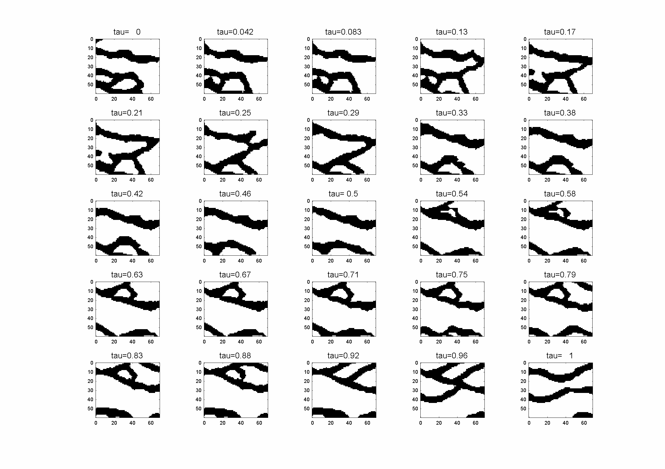 |
Example of applying the Probability Perturbation Method using S-GeMS