visim_init generate a reference data structure (equivalent of a VISIM parameter file) for unconditional simulation:

V=visim_init;
V=visim(V);
visim_plot_sim(V);

visim_init can optionally be called with a suggested geometry:

V=visim_init(1:1:50,1:2:200);
V=visim(V);
visim_plot_sim(V);

Finally, visim_init an existing VISIM structure can be passed, that will form the base of an update VISIM structure:

V=visim_init(1:1:50,1:2:200,V);
V=visim(V);
visim_plot_sim(V);

When visim_init is called, the gloval variance V.gvar is checked for consistency with the semivariogram model, and fixed appropriately such that the global variance is set to the total sill value of the specicied semivariogram. The tail values will also be checked for consistency if V.ccdf=1.

If V.ccdf=1, direct sequential simulation is performed. This enable the use of a non-Gaussian distribution of the subsurface parameters (the target distribution). The shape of the target distribution is given by the data found in the fileV.refhist.fname. The target distribution can be treated as either a continious or a discrete function usingV.refhist.do_discrete.

The following example will perform unconditional simulation with a trimodal target distribution assumed to be continious:

V=visim_init(1:1:61,1:1:61);
V.parfile='visim_example_dssim_cont_1.par';
d1=randn(1,2000)*sqrt(.2)+8;
d2=randn(1,1200)*sqrt(.1)+10;
d3=randn(1,2800)*sqrt(.1)+13;
d_target=[d1,d2,d3]';
V.refhist.fname='dssim_target.eas';
write_eas(V.refhist.fname,d_target); % write target distribution
V.ccdf=1;                 % use DSSIM
V.refhist.do_discrete=0;  % Assume continious target histogram
V.nsim=10;
V=visim_init(V); 
V.Va.it=3;     % Choose Gaussian semivariogram
V.Va.a_hmax=15; % correlation length (direction of max continuity)
V.Va.a_hmin=15; % correlation length (direction of min continuity)
V=visim(V);
figure(1);visim_plot_sim(V);
print_mul('visim_example_dssim_cont_sim');
figure(2);visim_plot_hist(V);
print_mul('visim_example_dssim_cont_hist');

The following example will perform unconditional simulation with a target distribution chosen as [1 10 10 40], asssmued to be continious:

V=visim_init(1:1:61,1:1:61);
V.parfile='visim_example_dssim_cont_2.par';
d_target=[1 10 10 40]';
V.refhist.fname='dssim_target_discrete.eas';
write_eas(V.refhist.fname,d_target); % write target distribution
V.ccdf=1;                 % use DSSIM
V.refhist.do_discrete=0;  % Assume continious target histogram
V.nsim=10;
V=visim_init(V); 
V.Va.it=3;     % Choose Gaussian semivariogram
V.Va.a_hmax=15; % correlation length (direction of max continuity)
V.Va.a_hmin=15; % correlation length (direction of min continuity)
V=visim(V);

figure(1);visim_plot_sim(V);
print_mul('visim_example_dssim_cont_1_sim');
figure(2);visim_plot_hist(V);
print_mul('visim_example_dssim_cont_1_hist');

The last DSSIM example is a example of unconditional simulation with a target distribution chosen as [1 10 10 40], asssmued to be discrete. This means that no other values than the ones given in the target distirbution can be simulated. This can be used for categorical simulation:

V=visim_init(1:1:61,1:1:61);
V.parfile='visim_example_dssim_discrete_1.par';
d_target=[1 10 10 40]';
V.refhist.fname='dssim_target_discrete.eas';
write_eas(V.refhist.fname,d_target); % write target distribution
V.ccdf=1;                 % use DSSIM
V.refhist.do_discrete=1;  % Assume continious target histogram
V.nsim=10;
V=visim_init(V); 
V.Va.it=3;     % Choose Gaussian semivariogram
V.Va.a_hmax=15; % correlation length (direction of max continuity)
V.Va.a_hmin=15; % correlation length (direction of min continuity)
V=visim(V);

figure(1);visim_plot_sim(V);
print_mul('visim_example_dssim_discrete_1_sim');
figure(2);visim_plot_hist(V);
print_mul('visim_example_dssim_discrete_1_hist');

Correlated data errors can be specified as an EAS formatted ascii file with the name datacov_[V.fout]. If for example the output file for visim.par is set to visim.out, then the file with correlated data errors should be name datacov_visim.out. If this file exist, correlated data errors are read from the file appropriately. If the file does not exist, UNcorrelated data errors are assumed, as given by the fourth column of the V.fvolsum.fname file.

VISIM can be used to solve any linear inverse problem, using both estimation and simulation. The function G_to_visim converts a linear inverse problem in Matlab format to a visim format:

load lsq_example.mat
V=G_to_visim(x,y,z,d_obs,G,Cd,m0);

% MAKE SURE THE KERNEL LOOKS OK
figure;
subplot(1,2,1);visim_plot_kernel(V); % All kernels
subplot(1,2,2);visim_plot_kernel(V,2); % the 2nd kernel

V.volnh.max=200; % MAX NUMBER OF VOLUMES TO USE
V.Va.a_hmax=0;
V.Va.a_hmin=0;

% Estimation using VISIM
V.nsim=0;
Vest=visim(V);

% Simulation using Matlab
V.nsim=10;
Vsim=visim(V);

% Estimation using Matlab
m0=zeros(V.nx*V.ny,1)+m0;
d0=G*m0;
Cm=V.gvar.*eye(V.nx*V.ny);
m_est = m0 +Cm*G'*inv(G*Cm*G' + Cd)*(d_obs-d0);
Cm_est = Cm - Cm*G'*inv( G*Cm*G' + Cd  )*G*Cm;

subplot(2,3,1);
imagesc(V.x,V.y,reshape(m_est,V.ny,V.nx));axis image
cax=caxis;
title_alt('LSQ mean',1)
subplot(2,3,2);
imagesc(V.x,V.y,Vest.etype.mean');axis image;caxis(cax)
title_alt('VISIM LSQ mean',2)
subplot(2,3,3);
imagesc(V.x,V.y,Vsim.etype.mean');axis image;caxis(cax)
title_alt('VISIM Etype mean',3)

subplot(2,3,4);
imagesc(V.x,V.y,reshape(diag(Cm_est),V.ny,V.nx));axis image
cax=caxis;
title_alt('LSQ var',4)
subplot(2,3,5);
imagesc(V.x,V.y,Vest.etype.var');axis image;caxis(cax)
title_alt('VISIM LSQ var',5)
subplot(2,3,6);
imagesc(V.x,V.y,Vsim.etype.var');axis image;caxis(cax)
title_alt('VISIM LSQ etype',6)

As VISIM conditions to linear average measurements of the model parameter space, VISIM can be used to draw samples from the a posteriori probability distribution linear inverse problems.

V=read_visim('visim_sgsim_cond_3.par');

V.nsim=100;

% Traditional conditional Gaussian simulation
Vseqsim=visim(V);
% Conditional simulation through error simulation
Verrsim=visim_errsim(V);

Calculating averaging kernels for cross borehole tomography

To deal with any kind of linear inverse problem in VISIM the averaging kernel describing the forward problem must be given

The averaging kernel is defined in two text files visim_volgeom.eas (defining the geometry of each average kernel) and visim_volsum.eas. (giving the observed average and measurement error for each defined volume average.

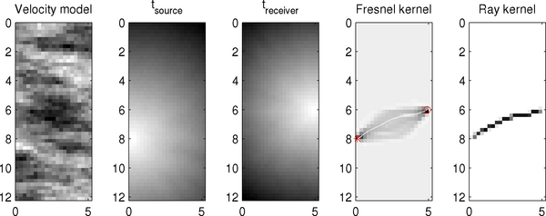
These two files can be calculated for tomography problems with arbitrary source-receiver geometry, and for a specific velocity model. Both the high frequency approximation to the wave equation, rays, and Fresnel zone based kernels can be generated using the visim_setup_punch

V=read_visim('sgsim_reference.par');
nx=V.nx;
ny=V.ny;
nz=V.nz;

m_ref=read_eas('visim_sgsim_refmod.eas');
m_ref=reshape(m_ref(:,3),ny,nx)';
% m_ref=zeros(nx,ny)+0.13;

S=linspace(1,11.5,7);
R=linspace(2,10,7);

[ss,rr]=meshgrid(S,R);

S=[ss(:).*0+.1 ss(:)];
R=[rr(:).*0+4.9 rr(:)];

type=1;  % [1]: Ray approximation, [2]: Fresnel zone based kernels
doPlot=1;% [0]: No visual progress, [1]: Plot all kernels as they are computed.

% CALCULATE GEOMETRY IN REF MODEL
[V_ray,G_ray]=visim_setup_punch(V,S,R,m_ref,[],[],'ref_rays',type,doPlot);
type=2;  % [1]: Ray approximation, [2]: Fresnel zone based kernels
[V_fre,G_fre]=visim_setup_punch(V,S,R,m_ref,[],[],'ref_frechet',type,doPlot);
  

See more info at the section called “visim_plot_kernel”

To visualize the generated averaging kernels use for example :

subplot(1,2,1)
visim_plot_kernel(V_ray);caxis([0 .1])
subplot(1,2,2)
visim_plot_kernel(V_fre);caxis([0 .1])

Now we compute the observed travel time from the refernce model and the current ray geometry

t_obs=G_ray*m_ref(:);
t_err=0.*t_obs.*.01;
[V_tomo]=visim_setup_punch(V,S,R,m_ref,t_obs,t_err,'tomo_ray',type,doPlot);

This generates the filename visim_tomo_ray.par. This parameter file can now be used to perform estimation and/or simulation :

V_tomo.cond_sim=3;   % condition to volume averages only (no point data)
V_tomo.nsim=100;     % 100 realizations
V_tomo.volh.max=100; % max 100 average data in the neighborhood.
V_tomo=visim(V_tomo);